Monetary analysis suggests that the global economy will weaken into early 2025, while inflation will continue to decline. A cyclical forecasting framework, on the other hand, points to the possibility of strong economic growth in H2 2025 and 2026.

Are the two perspectives inconsistent? A reconciliation could involve downside economic and inflation surprises in H2 2024 triggering a dramatic escalation of monetary policy easing. A subsequent pick-up in money growth would lay the foundation for a H2 2025 / 2026 economic boom.

How would equities perform in this scenario? Bulls would argue that any near-term weakness due to negative economic news would be swiftly reversed as policies eased and markets shifted focus to the sunlit uplands of H2 2025 / 2026.

More likely, a significant fall in risk asset prices would be necessary to generate easing of the required speed and scale, and a subsequent recovery might take time to gather pace.

Global six-month real narrow money momentum has recovered from a major low in September 2023 but remains weak by historical standards and fell back in May – see chart 1. The assessment here is that the decline into the 2023 low will be reflected in a weakening of global economic momentum in H2 2024.

Chart 1
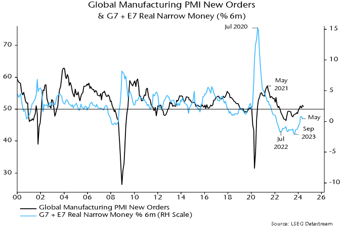
Chart 1 showing Global Manufacturing PMI New Orders and G7 plus E7 Real Narrow Money

A counter-argument is that a typical lead-time between lows in real money and economic momentum historically has been six to 12 months. On this basis, negative fall-out from the September 2023 real money momentum low should be reaching a maximum now, with the subsequent recovery to be reflected in economic acceleration in late 2024.

The latter interpretation is consistent with the consensus view that a sustainable economic upswing is under way and will gather pace as inflation progress allows gradual monetary policy easing.

The pessimistic view here reflects three main considerations. First, economic acceleration now would imply an absence of any negative counterpart to the September 2023 real money momentum low – historically very unusual.

Secondly, the lag between money and the economy has recently been at the top end of the historical range, suggesting that a significant portion of 2023 monetary weakness has yet to feed through.

Highs in real money momentum in August 2016 and July 2020 preceded highs in global manufacturing PMI new orders by 16 and 10 months respectively, while a low in May 2018 occurred a year before a corresponding PMI trough – chart 2.

Chart 2
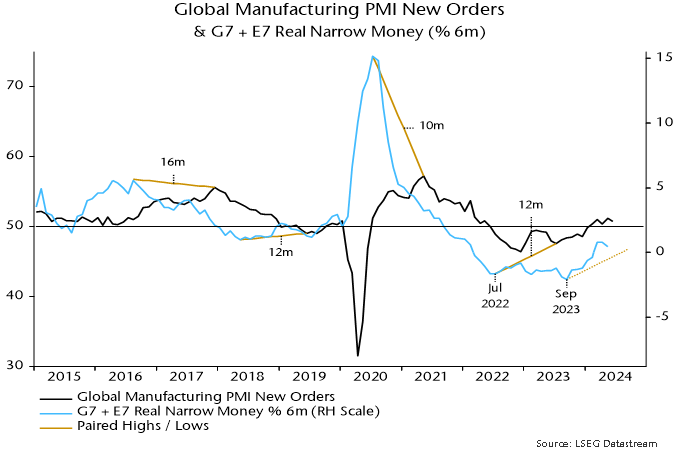
Chart 2 showing Global Manufacturing PMI New Orders and G7 plus E7 Real Narrow Money

So a PMI low associated with the September 2023 real money momentum trough could occur as late as January 2025.

Thirdly, stock as well as flow considerations have been important for analysing the impact of money on the economy in recent years, and a current shortfall of real narrow money from its pre-pandemic trend may counteract a positive influence from the (tepid) recovery in momentum since September 2023 – chart 3.

Chart 3

Chart 3 showing Ratio of G7 and E7 Real Narrow Money to Industrial Output and 1995 to 2019 Log-Linear Trend

The decline in real money momentum into the September 2023 low began from a minor peak in December 2022, suggesting that the PMI – even allowing for a longer-than-normal lag – should have peaked by early 2024. Global manufacturing PMI new orders rose into March and made a marginal new high in May. However, two indicators displaying a significant contemporaneous correlation with PMI new orders historically – PMI future output and US ISM new orders – peaked in January. The future output series fell sharply in June, consistent with the view that another PMI downturn is starting – chart 4.

Chart 4

Chart 4 showing Global Manufacturing PMI New Orders and Global Manufacturing PMI Future Output / US ISM Manufacturing New Orders

Signs of weakness are also apparent under the hood of the services PMI survey. Overall new business has been boosted by financial sector strength, reflecting buoyant markets, but the consumer services component fell to a six-month low in June – chart 5.

Chart 5

Chart 5 showing Global Services PMI New Business

Could a weakening of economic momentum in H2 2024 snowball into a deep / prolonged recession? The cycles element of the forecasting process used here suggests not.

Severe / sustained recessions occur when the three investment cycles – stockbuilding, business capex and housing – move into lows simultaneously. The most recent troughs in the three cycles are judged to have occurred in Q1 2023, 2020 and 2009 respectively. Allowing for their usual lengths (3-5, 7-11 and 15-25 years), the next feasible window for simultaneous lows is 2027-28 – chart 6. Cycle influences should be positive until then.

Chart 6

Chart 6 showing Actual and Possible Cycle Trough Years

Major busts associated with triple-cycle lows, indeed, are usually preceded by economic booms. Such booms often involve policy shifts that super-charge positive cyclical forces. The 1987 stock market crash, for example, triggered rate cuts by the Fed and other central banks that magnified a late 1980s housing cycle peak.

Could significant policy easing in H2 2024 / H1 2025 similarly catalyse a H2 2025 / 2026 boom? Such a policy shift, on the view here, is plausible because negative economic news into early 2025 is likely to be accompanied a melting of inflation concerns.

The latter suggestion is based on the monetarist rule-of-thumb that inflation follows money trends with a roughly two-year lag. G7 broad money growth of about 4.5% pa is consistent with 2% inflation. Annual growth returned to this level in mid-2022, reflected in a forecast here that inflation rates would move back to target in H2 2024 – chart 7.

Chart 7
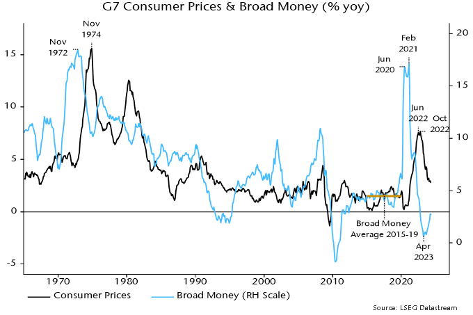
Chart 7 showing G7 Consumer Prices and Broad Money

The forecast is within reach. Annual US PCE and Eurozone CPI inflation rates were 2.5% in May and June respectively, with a fall to 2% in prospect by end-Q3 on reasonable assumptions for monthly index changes. UK CPI inflation has already dropped to 2.0%.

G7 annual broad money growth continued to decline into 2023, reaching a low of 0.6% in April 2023 and recovering gradually to 2.7% in May 2024. The suggestion from the monetarist rule, therefore, is that inflation rates will move below target in H1 2025 and remain low into 2026.

Central banks have been focusing on stickier services inflation, neglecting historical evidence that services prices lag both food / energy costs and core goods prices. Those relationships, and easing wage pressures, suggest that services resilience is about to crumble, a possibility supported by a sharp drop in the global consumer services PMI output price index in June to below its pre-pandemic average – chart 8.

Chart 8
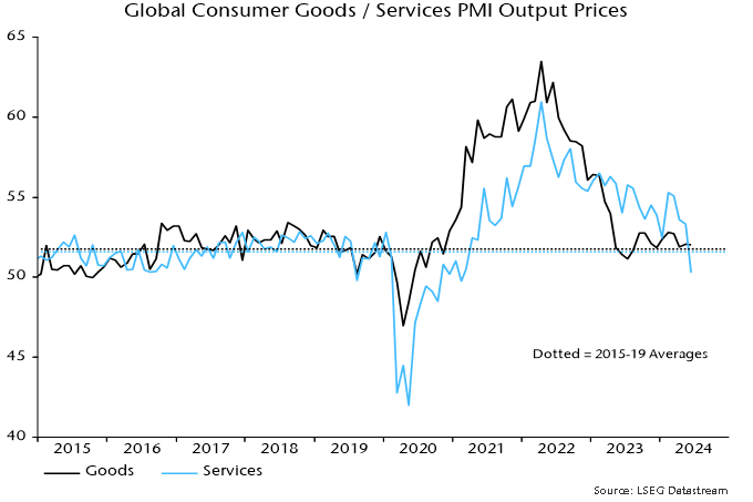
Chart 8 showing Global Consumer Goods / Services PMI Output Prices

The approach here uses two flow measures of global “excess” money to assess the monetary backdrop for equity markets: the gap between global six-month real narrow money and industrial output momentum, and the deviation of annual real money growth from a long-term moving average.

The two measures turned negative around end-2021, ahead of 2022 market weakness, but remained sub-zero as global indices rallied to new highs in H1 2024. The latter “miss” may be attributable to a money stock overshoot shown in chart 3 – the flow measures of excess money may have failed to capture the deployment of existing precautionary money holdings.

Still, the MSCI World index in US dollars outperformed dollar deposits by only 3.9% between end-2021 and end-June 2024, with the gain dependent on a small number of US mega-caps: the equal-weighted version of the index underperformed deposits by 8.4% over the same period.

What now? The money stock overshoot has reversed. The first excess money measure has recovered to zero but the second remains significantly negative. Mixed readings have been associated with equities underperforming deposits on average historically, with some examples of significant losses. Caution still appears warranted.

An obvious suggestion based on the economic scenario described above is to overweight defensive sectors. Non-tech cyclical sectors gave back some of their outperformance in Q2 but are still relatively expensive by historical standards, apparently discounting PMI strength – chart 9.

Chart 9
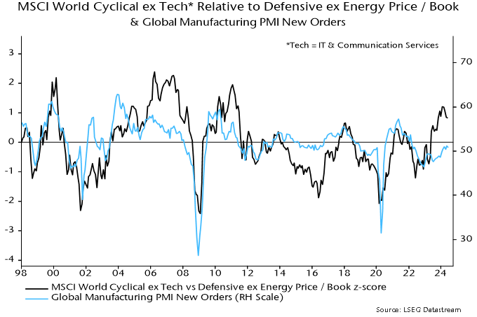
Chart 9 showing MSCI World Cyclical ex Tech* Relative to Devensive ex Energy Price/Book and Global Manufacturing PMI New Orders

Accelerated monetary policy easing could be favourable for EM equities, especially if associated with a weaker US dollar. Monetary indicators are promising. EM equities have outperformed historically when real narrow money growth has been higher in the E7 than the G7 and the first global excess money measure has been positive – chart 10. The former condition remains in place and the second is borderline.

Chart 10

Chart 10 showing MSCI EM Cumulative Return vs MSCI World and "Excess" Money Measures

Un billet de dix dollars canadiens sur un fond de billets

Le présent résumé jette un éclairage sur l’évolution du taux de change du dollar canadien par rapport au dollar américain à l’ère moderne. La figure 1 montre le niveau des taux de change de fin de mois de 1953 au 31 mars 2024.

Figure 1 : Historique du taux de change du dollar canadien par rapport au dollar américain


1953-1960 Pendant la plus grande partie de la période allant de 1953 à 1960, le dollar canadien a oscillé entre 1,02 $ US et 1,06 $ US. Son point culminant a été 1,0614 $, atteint le 20 août 1957. Jusqu’en 2007, on considérait que c’était là le niveau le plus élevé atteint par le dollar canadien par rapport au dollar américain à l’ère moderne. Le dollar canadien valait 2,78 $ US en 1864, au moment de la guerre civile américaine, mais, à l’époque, il était indexé sur l’or, une pratique que les États-Unis avaient déjà abandonnée.
1961-1969 Au début des années 1960, le gouverneur de la Banque du Canada, James Coyne, et le premier ministre de l’époque, John Diefenbaker avaient des vues différentes sur le sujet de l’économie. Le gouvernement était partisan d’une politique expansionniste, alors que Coyne souhaitait maintenir une politique de l’argent rare. Coyne en vint à remettre sa démission, et, en mai 1962, le gouvernement adopta un taux de change fixe, attribuant au dollar canadien une valeur de 92,5 cents US, susceptible de varier de 1 % à la hausse ou à la baisse.
1970-1972 En mai 1970, devant la montée de l’inflation et la flambée des salaires, le gouvernement Trudeau décida de laisser flotter le dollar canadien. Ce dernier s’orienta à la hausse, pour atteindre la parité avec le dollar américain en 1972.
1974 Le 24 avril 1974, le dollar canadien se hissait à 1,0443 $ US. Il s’agissait du niveau le plus élevé atteint depuis le début de la plus récente période de flottement, et il allait s’écouler 30 ans avant que le dollar canadien regagne un tel niveau.
1976- 1986 En novembre 1976, René Lévesque fut élu premier ministre du Québec avec un programme qui comportait le projet de faire l’indépendance du Québec. Il s’ensuivit un repli du dollar canadien qui se poursuivit pendant le reste des années 1970 et pendant la première moitié des années 1980. Cette période fut marquée par une montée de l’inflation et des taux d’intérêt. Le taux directeur de la Banque du Canada a atteint 21,2 % en 1981 et le dollar canadien a plongé vers un creux historique de 69,13 cents américains le 4 février 1986.
1987- 1997 Le dollar canadien s’apprécia pendant la dernière partie des années 1980 et au début des années 1990; le 4 novembre 1991, il atteignit 89,34 cents US. Ce fut son niveau le plus élevé de la décennie 1990.
1998-2002 Les déficits budgétaires, le recul des prix des matières premières et les conséquences de la crise internationale de 1998 dans les pays émergents de la Russie et de l’Amérique latine entraînèrent le dollar à la baisse. Le 21 janvier 2002, le dollar canadien chuta au plus bas niveau de son histoire face au dollar américain, à 61,79 cents US. À ce niveau, il fallait débourser 1,62 $ CA pour obtenir 1 $ US.
2003- 2006 De 2003 à 2006, le dollar canadien se redressa fortement à la faveur d’une bonne conjoncture économique mondiale qui fit grimper les prix des exportations canadiennes de matières premières et il franchit la barre des 90 cents US.
2007 Le 20 septembre 2007, le dollar canadien atteignit la parité avec le dollar américain pour la première fois depuis 31 ans; il avait progressé de 62 % en moins de six ans, en partie grâce aux prix élevés du pétrole et d’autres matières premières. Le dollar canadien fut désigné « personnalité canadienne de l’année 2007 » par l’édition canadienne du magazine Time.
2008- 2009 Le dollar canadien se maintint au voisinage de la parité au premier semestre 2008, avant de s’infléchir à la baisse, pour finalement glisser sous la barre des 80 cents US.
2010 Après un vif rebond, le dollar canadien atteignit de nouveau la parité pour la première fois en 20 mois en avril 2010.
2011 Au plus fort du boom des matières premières, le dollar canadien a atteint 1,06 $ US le 21 juillet 2011. Il amorça alors sa chute la plus rapide de l’ère moderne sur fond de brutal décrochage des matières premières.
2016 Le dollar canadien chuta à 68,68 cents US le 19 janvier 2016, à 7 cents US environ de son creux record, avant de repartir à la hausse face au billet vert pour finir l’année à 74,57 cents US.
2017- 2024 Les fluctuations de change ont été quelque peu modérées depuis 2016, bien que le dollar canadien soit redescendu pour atteindre la barre des 70 cents US en mars 2020 au début de la pandémie de COVID-19. Le dollar canadien s’est par la suite raffermi et s’est établi à 73,90 cents américains à la fin de mars 2024.


La figure 2 montre la variation des taux de change depuis 1970 et illustre donc le contexte associé aux fluctuations du dollar canadien par rapport au dollar américain à l’ère moderne.

Figure 2 : Taux de change $ CA/$ US


Les trois baisses du dollar canadien à partir d’un sommet jusqu’à un creux ont toutes été d’un peu plus de 30 %. Les deux premières baisses ont duré environ 10 ans, tandis que la plus récente a été la baisse la plus rapide, en raison en partie de l’effondrement brutal des prix du pétrole.

Depuis le dernier creux de 2016, le dollar canadien continue de fluctuer dans une fourchette relativement étroite, et ce, malgré l’incertitude associée à la pandémie de COVID-19 et les niveaux élevés actuels de l’inflation. Le dollar canadien devrait descendre sous la barre des 68,68 cents américains pour atteindre ce qui était considéré comme le creux de la dernière baisse.

Sources : Banque du Canada, CBC, Globe & Mail.

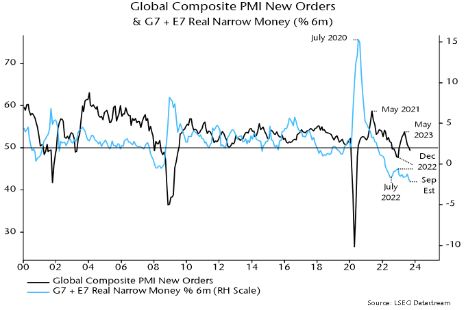
Global six-month real narrow money momentum – a key leading indicator in the forecasting approach employed here – is estimated to have fallen to another new low in September. Real money momentum has led turning points in global PMI new orders by an average 6-7 months historically, so the suggestion is that a recent PMI slide will extend through end-Q1 – see chart 1.

Chart 1

Chart 1 showing Global Composite PMI New Orders & G7 + E7 Real Narrow Money (% 6m)

The September real narrow money estimate is based on monetary data for countries with a two-thirds weight in the global (i.e. G7 plus E7) aggregate and CPI data for a higher proportion.

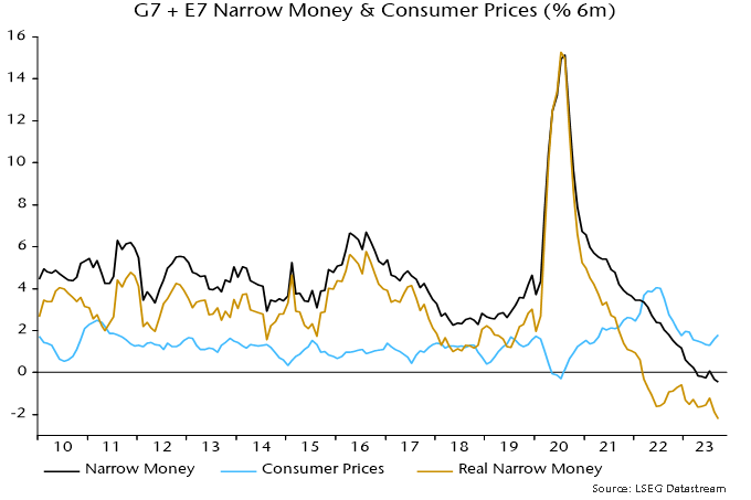
The estimated September fall reflects additional nominal money weakness coupled with a further oil-price-driven recovery in six-month CPI momentum – chart 2.

Chart 2

Chart 2 showing G7 + E7 Narrow Money & Consumer Prices (% 6m)

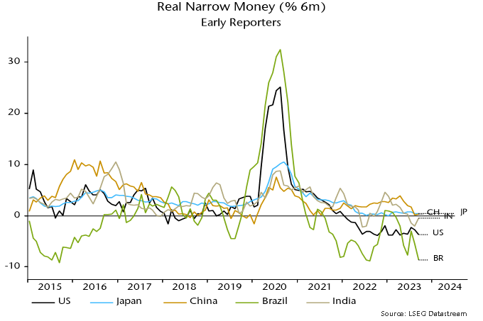
Among countries that have released September data, six-month real narrow money momentum fell in the US and Brazil, was little changed in China / Japan and recovered in India (because inflation reversed lower after a food-driven spike) – chart 3.

Chart 3

Chart 3 showing Real Narrow Money (% 6m) Early Reporters

Real narrow money momentum is primarily a directional indicator but the current extreme negative reading seems unlikely to be consistent with hopes of a “soft landing”.

One argument for the latter is that a drag on manufacturing trade and activity from a downswing in the stockbuilding cycle is coming to an end, to be followed by a recovery into 2024. A trough by end-2023 has long been the base case here but monetary weakness suggests that the cycle will bump along the bottom rather than enter an upswing.

More precisely, an initial boost from an ending of destocking may fizzle as the usual multiplier effects are offset by slower or falling final demand due to monetary restriction.

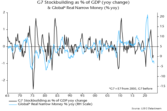
Stockbuilding cycle upswings historically were always preceded by a recovery (of variable magnitude) in global real narrow money momentum – chart 4.

Chart 4

Chart 4 showing G7 Stockbuilding as % of GDP (yoy change) & Global* Real Narrow Money (% yoy) *G7 + E7 from 2005, G7 before

Current conditions are reminiscent of the early 1990s, when real money momentum remained near its low between H2 1989 and H1 1991 and an easing of a stockbuilding drag in 1990 was followed by a relapse into 1991. Monetary weakness, on that occasion, appears to have resulted in an extended cycle, with a final low in Q2 1991 occurring 4 1/2 years after the previous trough in Q4 1986 versus an average cycle length of 3 1/3 years. For comparison, the current cycle started in Q2 2020 so has recently moved beyond the 3 1/3 year average.

A bottoming out of the global stockbuilding cycle could be associated with a near-term recovery in manufacturing survey indicators. Money trends suggest that any revival will be modest / temporary and offset by wider economic weakness. 

Economic news has been unusually mixed since end-2021, with GDP weakness contrasting with labour market strength and manufacturing deterioration offset by services resilience. Confusing signals have contributed to market hopes of a “soft landing”. 

Sectoral and regional divergences may persist in H2 2023. The expectation here is that manufacturing survey weakness will abate but labour market data will worsen significantly. Money trends continue to cast strong doubt on soft landing hopes. Europe is likely to underperform the US. 

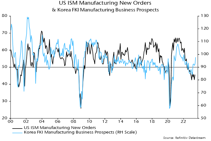
The US ISM manufacturing new orders index – a widely watched indicator of industrial momentum – hit a low of 42.5 in January and retested this level in May before recovering to 45.6 in June. 

Reasons for expecting a further rise include: 

  • The index has been in the 40s since September 2022 and the mean duration of sub-50 periods historically was eight months (ignoring episodes of three months or less). 
  • The global stockbuilding cycle remains on track to bottom out during H2 2023 and lows historically were usually preceded by a recovery in US / global manufacturing new orders. 
  • Recent price falls for raw materials and other production inputs may further incentivise firms to step up purchasing to maintain or replenish inventories.

Korean manufacturing is a bellwether of US / global trends and the latest Federation of Korean Industries survey reported a marked improvement in optimism, consistent with ISM new orders moving back above 50 – see chart 1. 

Chart 1

Chart 1 showing US ISM Manufacturing New Orders & Korea FKI Manufacturing Business Prospects

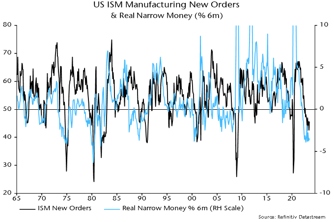
Sustained recoveries in ISM new orders from the mid 40s into expansionary territory historically occurred against a backdrop of positive and / or rising six-month real narrow money* momentum. Current trends are unfavourable, with momentum still significantly negative and moving sideways – chart 2. 

Chart 2

Chart 2 showing US ISM Manufacturing New Orders & Real Narrow Money (% 6m)

Examples of recoveries to above 50 without a supportive monetary backdrop include 1970 and 1989-90. In both cases the rise was modest (peaking below 55), short-lived and followed by a decline to a lower low. The recovery in 1970 occurred within an NBER-defined recession and in 1989-90 just before one. 

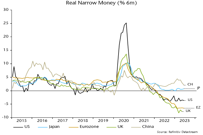
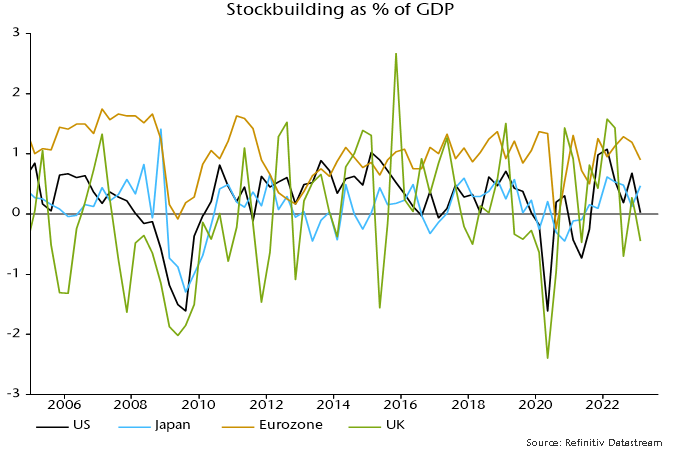
An ISM rebound might not be mirrored by much if any revival in European manufacturing surveys. Money trends are even weaker than in the US, while the stockbuilding adjustment started later in the Eurozone and probably has further to run – charts 3 and 4. 

Chart 3

Chart 3 showing Real Narrow Money (% 6m)

Chart 4

Chart 4 showing Stockbuilding as % of GDP

*Narrow money definition used here = M1A = currency + demand deposits.

Beautiful view of a Puerto Vallarta beach on the Pacific coast of Mexico.

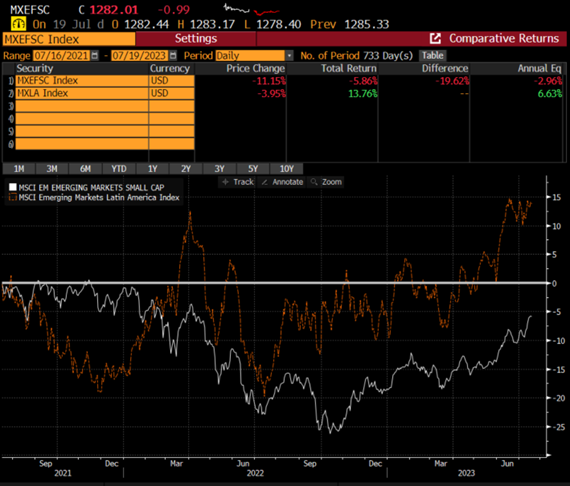
Latin America has outperformed other emerging markets over the past two years and this positive performance can be attributed to several key factors. However, the challenge lies in sustaining this momentum and ensuring it is not merely temporary.

MSCI World Small Cap Index vs MSCI Emerging Markets Latin America Index, 2021 to 2023

Graph showing the outperformance of the Latin America small cap index relative to its global peers between June 2021 and June 2023.

Source: Bloomberg

Notably, the combination of currency rallies among some Latin American countries and an emerging markets rally is uncommon. Reasons for this mismatch include:

  • Latin America leads the way in interest rate hikes worldwide. Starting in the first half of 2021, Chile and Brazil raised rates, helping control inflation levels, although they are still high but manageable. Chile will likely start its easing process next week, followed by Brazil within the year. This has boosted their respective stock markets, which were already undervalued in our view.
  • Additionally, Mexico has benefitted from the “nearshoring” theme. Nearshoring is nothing new to local investors, having been present in the region for decades. What is new is the level of intensity and amount of investment expected over the next three to five years. This has resulted in increased earnings per share (EPS) of 15% to 20% CAGR in the near term for some Mexican companies, outperforming the MSCI Emerging Markets Small Cap Index and contributing to higher valuations in Mexico’s market compared to its Latin American peers. However, there are questions about whether Mexico’s growth is comparable to its peers or to countries like Indonesia or Vietnam that are also heavily dependent on US imports.
  • Commodities also play a significant role in the region’s performance. Despite a global slowdown, certain commodities, like copper, have maintained high prices due to supply constraints. We believe the anticipated electric vehicle (EV) boom will further drive copper demand, ensuring a deficit in the market from 2026 onwards. For example, every EV, which weigh approximately two tons each, consumes around 60 additional kilos of copper.
  • Furthermore, the region has demonstrated better fiscal discipline, with countries like Chile and Mexico ending 2022 with fiscal surpluses or manageable deficits, respectively. This responsible fiscal approach has also supported their currencies. There is always the potential for Brazil to surprise on the downside due to its high fiscal spending and debt levels; however, the country has seen no “disruptive” events lately.
  • US rates hikes have favoured value over growth factors in emerging markets, benefitting markets like Latin America’s over countries perceived as growth-driven, such as Korea or India.
  • Innovation has not been a main driver for Latin America, but that is starting to slowly change. Moreover, the market has begun recognizing and crediting good companies with sustained growth expectations, which has historically been uncommon in the region. This trend in recognizing innovation and good companies is crucial for bottom-up investors like us who prioritize companies with solid balance sheets, strong cash flow generation and sustained competitive advantages. More Latin American companies have started to share these characteristics.

Latin America is still a small region relative to the rest of the world and it is dominated by, and benefits from, global trends, even though its politics are not always market friendly. However, sustained positive factors like the commodities momentum and nearshoring may make global investors more indifferent to the region’s internal dynamics.

What needs to happen for long-term compounder growth stories to emerge, like Nestle in India or TSMC in Taiwan? To maintain sustainable growth, we believe the region needs to align with external factors and foster strong domestic sectors and companies that promote growth. Improving innovation and adapting to rapidly changing environments are also key. For example, the financial sector in Mexico and Chile remains solid, while the transport-logistics sector in Mexico offers interesting opportunities. Brazil’s large population presents significant potential for emerging middle-class growth, creating opportunities in various sectors.

Latin America has growth engines and the key is to identify the best companies capable of maintaining a sustained differentiation over time. By focusing on these opportunities, our portfolio is well-positioning to capture their potential growth.

Company example

JSL (JSLG3 BZ) has the largest portfolio of logistics in Brazil, with long expertise operating in a variety of sectors and a nationwide scale of services. The company has long-lasting business relationships with clients that operate in several economic sectors, including pulp and paper, steel, mining, agribusiness, automotive, food, chemical and consumer goods, among others. JSL also has a unique position in the Brazilian highway logistics market, as leader for 19 years and much larger than its nearest competitor.

The logistics industry in Brazil is highly fragmented, with a high level of informality and low capitalization among players. This creates opportunities for further consolidation, especially for companies with structured businesses. According to Citibank, the top 10 companies have close to a 2% market share. JSL has roughly 1% market share (almost 5x the second-largest player) and is well placed to continue consolidating the industry. JSL also has a favourable M&A track record, which has been a growth driver in recent years. JSL has acquired seven companies since its re-IPO in October 2020 implying c20% annual organic growth and c60% EBITDA growth considering the acquisitions, maintaining strong returns. 

We also expect JSL to continue expanding its ROIC going forward, driven by the ongoing consolidation of new acquisitions into JSL’s financials, the company’s strategy to becoming a less capital intensive, asset light business, and strong revenue growth to maintain gaining scale and operating leverage. The logistics industry offers a lot of opportunities to implement tech-driven innovation, and we see JSL well-positioned to use its sector platform and status as a leading tech player. The stock has performed very well this year, partially driven by rate cut expectations and also strong earnings. We expect the company to continue delivering good results in upcoming quarters amid a highly fragmented sector, creating both organic and inorganic growth engines.

The Sahm rule states that the (US) economy is likely to be in recession if a three-month moving average of the unemployment rate is 0.5 pp or more above its minimum in the prior 12 months. 

The rule identified all 12 US recessions since 1950 but gave two false positive signals based on current (i.e., revised) unemployment rate data (1959 and 2003) and four based on real-time data (additionally 1967 and 1976). 

The signal occurred after the start date of the recession in all 12 cases, with a maximum delay of seven months* (in the 1973-75 recession). 

The Sahm condition hasn’t yet been met in the US – the unemployment rate three-month average was 3.6% in June versus a 12-month minimum of 3.5%. 

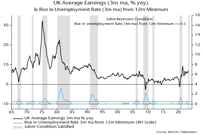
The rule has, however, triggered a warning in the UK, where the jobless rate averaged 4.0% over March-May, up from 3.5% over June-August 2022. 

UK Sahm rule warnings occurred on nine previous occasions since 1965, six of which were associated with GDP contractions. 

The Sahm signal is another indication that the UK economy is already in recession – see previous post – but a stronger message is that earnings growth is about to slow. 

Annual growth of average earnings fell after the Sahm signal in eight of the nine cases, the exception being the 2020 covid recession, when earnings numbers were heavily distorted by composition effects – see chart 1. 

Chart 1

Chart 1 showing UK Average Earnings (3m ma, % yoy) & Rise in Unemployment Rate (3m ma) from 12m Minimum

Previous generations of monetary policy-makers understood the dangers of basing decisions on the latest inflation and / or earnings data, which reflect monetary conditions 18 months or more ago. 

The current reactive approach, apparently endorsed by the economics consensus, may partly reflect mythology about a 1970s “wage / price spiral”. Rather than causing each other, high wage growth and inflation were dual symptoms of sustained double-digit broad money expansion. 

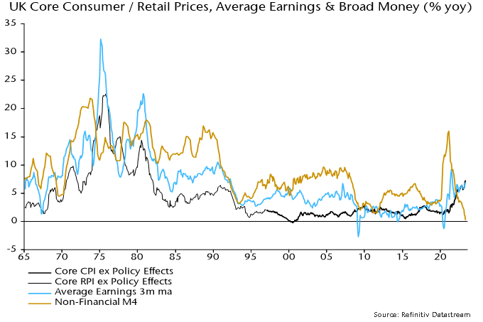
The monetarist case is summarised by chart 2, showing that earnings growth is almost coincident with core inflation whereas broad money expansion displays a long lead. (The correlations with core inflation are maximised with lags of four months for earnings growth and 24 months for money growth.) 

Chart 2 

Chart 2 showing UK Core Consumer / Retail Prices, Average Earnings & Broad Money (% yoy)

Recent monetary weakness argues that core inflation and wage growth will be much lower by late 2024; the Sahm rule signals that the decline is about to start.

*Eight months taking into account a one-month reporting lag.

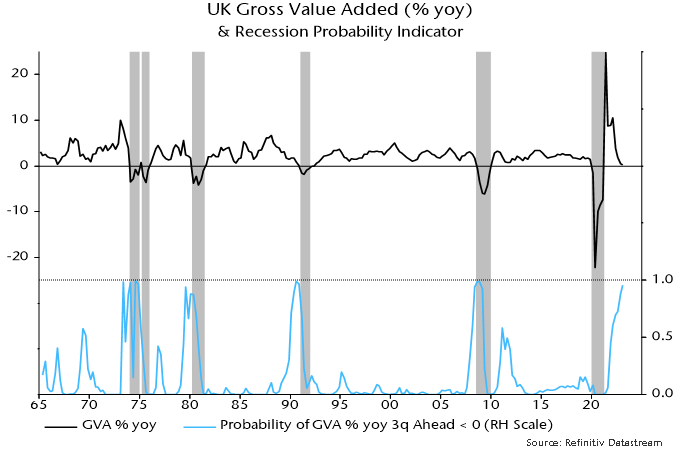
A recession likelihood gauge placing weight on monetary variables indicates a high probability of a contraction in UK GDP / gross value added (GVA) over the remainder of 2023. 

The indicator, regularly referenced in posts here, is based on a model that generates projections for the four-quarter change in GVA three quarters in advance using current and lagged values of a range of monetary and financial inputs. 

Using data up to June 2022, the model assigned a 70% probability to the four-quarter change in GVA being negative in Q1 2023. The current ONS estimate of this change is +0.2%. 

UK Gross Value Added (% yoy) & Recession Probability Indicator. Source: Refinitiv Datastream.

The probability reading rises to 96% incorporating data through March 2023, i.e. there is a 96% likelihood of the four-quarter change in GVA in Q4 2023 being negative, according to the model. 

The statistical analysis underlying the model indicates that GDP prospects are significantly influenced by movements in real narrow money (non-financial M1) and real corporate broad money (M4). Six-month rates of change of these measures have moved deeper into negative territory since mid-2022. 

The model’s increased pessimism also reflects a deepening inversion of the yield curve and falling real house prices. Other inputs include credit spreads and local share prices, which have yet to display recession-scale weakness.

DM flash results released last week suggest that the global manufacturing PMI new orders index fell sharply in June, having moved sideways in April and May following a Q1 recovery – see chart 1. 

Chart 1

Global Manufacturing PMI New Orders, & G7 + E7 Real Narrow Money (% 6m). Source: Refinitiv Datastream.

The relapse is consistent with a decline in global six-month real narrow money momentum from a local peak in December 2022. A recovery in real money momentum during H2 2022 had presaged the Q1 PMI revival. 

Real narrow money momentum is estimated to have fallen again in May, based on partial data, suggesting further PMI weakness into late 2023. 

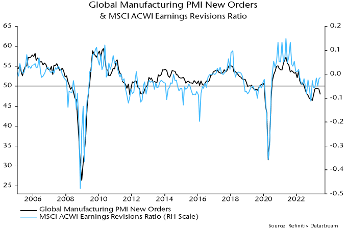
The global earnings revisions ratio has been contemporaneously correlated with manufacturing PMI new orders historically but remained at an above-average level in June, widening a recent divergence – chart 2. 

Chart 2

Global Manufacturing PMI New Orders, & MSCI ACWI Earnings Revisions Ratio. Source: Refinitiv Datastream.

Based on monetary trends, a reconvergence is more likely to occur via weaker earnings revisions than a PMI rebound. 

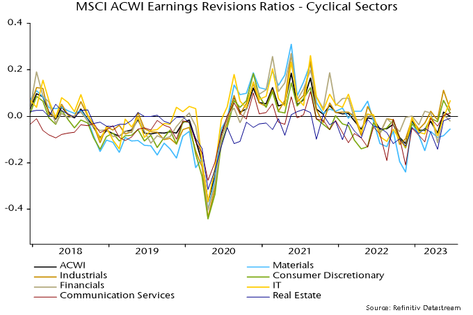
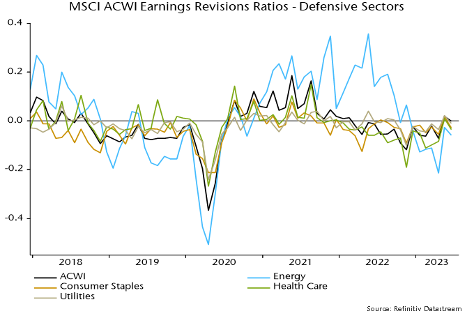
Charts 3 and 4 show that revisions resilience has been driven by cyclical sectors – in particular, IT, industrials and consumer discretionary. Notable weakness has been confined to the materials sector. Cyclical sectors may be at greater risk of downgrades if the global revisions ratio heads south. 

Defensive sector revisions have underperformed recently but are likely to be less sensitive to economic weakness. 

Chart 3

MSCI ACWI Earnings Revisions Ratios - Cyclical Sectors. Source: Refinitiv Datastream.

Chart 4

MSCI ACWI Earnings Revisions Ratios - Defensive Sectors. Source: Refinitiv Datastream.

The positive divergence of earnings revisions from the PMI may reflect firms’ ability to push through price increases to compensate for slower volumes. The deviation of the global revisions ratio (rescaled) from manufacturing PMI new orders – i.e. the gap between the blue and black lines in chart 2 – has displayed a weak positive correlation with the PMI output price index historically (contemporaneous correlation coefficient = +0.41). 

Any earnings support from pricing gains is now going into reverse: the output price index has crashed from an April 2022 peak of 63.8 to 49.8 in May, with DM flash results suggesting a further fall last month.

Why believe the “monetarist” forecast that recent G7 monetary weakness will feed through to low inflation in 2024-25? 

Monetary trends correctly warned of a coming inflationary upsurge in 2020 when most economists were emphasising deflation risk. 

The forecast of rapid disinflation is on track in terms of the usual sequencing, with commodity prices down heavily, producer prices slowing sharply and services / wage pressures showing signs of cooling. 

A further compelling consideration is that the monetary disinflation expected in G7 economies has already played out in emerging markets. 

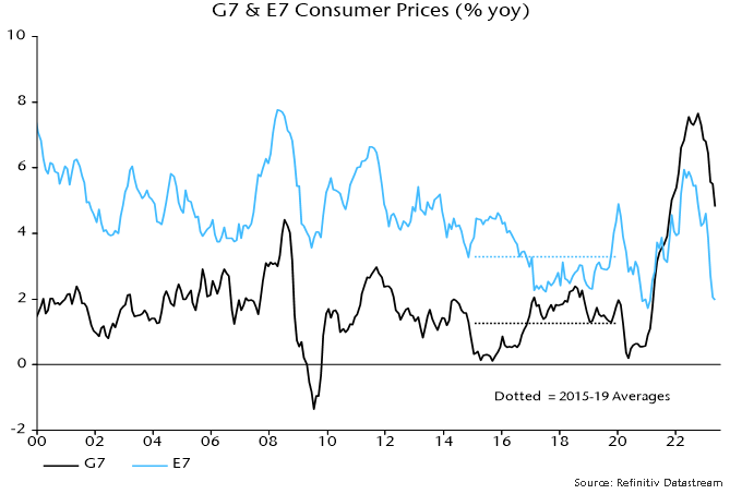
A GDP-weighted average of CPI inflation rates in the “E7” large emerging economies* crossed below its pre-pandemic (i.e. 2015-19) average in March, falling further into May – see chart 1. 

Chart 1

G7 & E7 Consumer Prices (% yoy). Source: Refinitiv Datastream.

The E7 average is dominated by China but inflation rates are also below or close to pre-pandemic levels in Brazil, India and Russia. 

Inflation rose by much less in the E7 than the G7 in 2021-22, opening up an unprecedented negative deviation that has persisted. 

The recent plunge in the E7 measure reflects a significant core slowdown as well as lower food / energy inflation. 

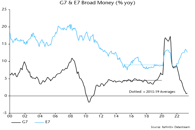
The divergent G7 / E7 experiences are explained by monetary trends. Annual broad money growth rose by much less in the E7 than the G7 in 2020 and returned to its pre-pandemic average much sooner – chart 2. 

Chart 2

G7 & E7 Broad Money (% yoy). Source: Refinitiv Datastream.

E7 broad money growth crossed below the pre-pandemic average in May 2021. CPI inflation, as noted, followed in March 2023, i.e. consistent with the monetarist rule of thumb of a roughly two-year lead from money to prices. 

G7 broad money growth crossed below its pre-pandemic average in August 2022 and has yet to bottom, suggesting a return of inflation to average in summer 2024 and a subsequent undershoot. 

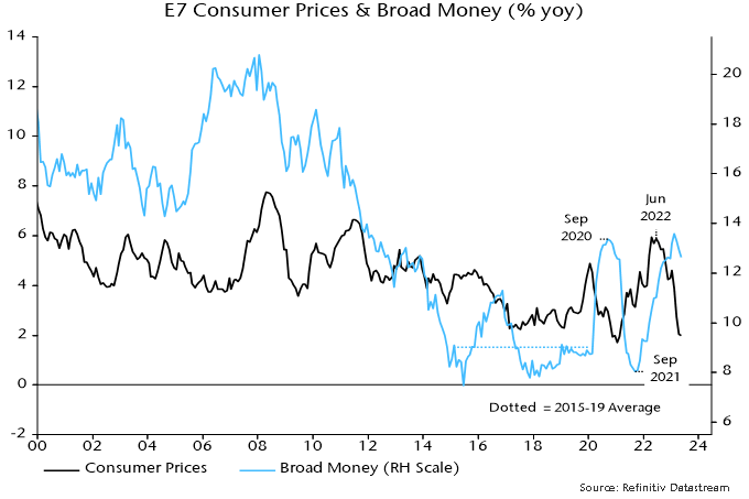
E7 disinflation, however, may be close to an end. Annual broad money growth has recovered strongly from a low in September 2021, signalling a likely inflation rebound during 2024 – chart 3. Broad money acceleration has been driven by China, Russia and Brazil. 

Chart 3

E7 Consumer Prices & Broad Money (% yoy). Source: Refinitiv Datastream.

E7 annual broad money growth is around the middle of its longer-term historical range and has eased since February. Chinese numbers may have been temporarily inflated by a shift in banks’ funding mix in favour of deposits. 

The expected rise in E7 inflation may not extend far but restoration of a positive E7 / G7 differential is likely in 2024.

*E7 defined here as BRIC + Korea, Mexico, Taiwan.

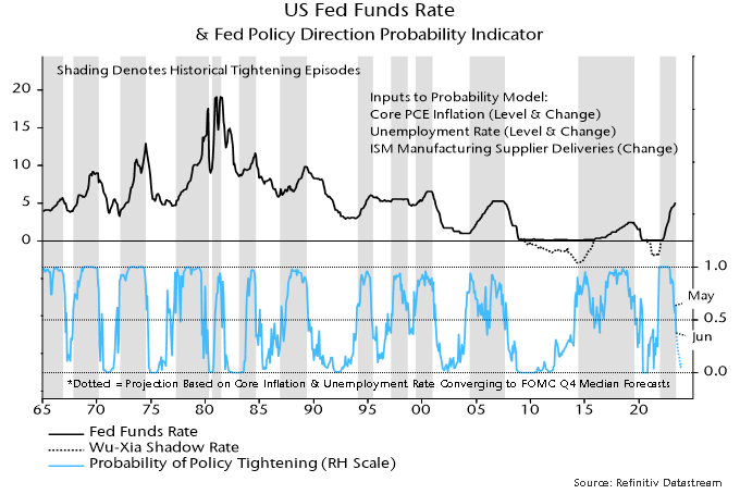
The FOMC’s updated economic forecast for the remainder of 2023 is inconsistent with Committee members’ median expectation of a further 50 bp rise in official rates during H2, according to a model based on the Fed’s past behaviour. Policy is more likely to be eased than tightened if the forecast plays out. 

The model estimates the probability of the Fed tightening or easing each month from current and lagged values of core PCE inflation, the unemployment rate and the ISM supplier deliveries index, a measure of production bottlenecks. It provides a simple but satisfactory explanation of the Fed’s historical decision-making, i.e. the probability estimate was above 50% in most tightening months and below 50% in most easing months – see chart. 

US Fed Funds Rate & Fed Policy Direction Probability Indicator.

The probability of the Fed tightening at yesterday’s meeting had been estimated by the model at 36%, the first sub-50% reading since September 2021. (The FOMC started to taper QE at the following meeting in November.) 

The FOMC’s median forecast for core PCE inflation in Q4 was revised up to 3.9% from 3.6% previously (currently 4.7%). The unemployment rate forecast was lowered to 4.1% from 4.5% (currently 3.7%). 

The model projections shown in the chart assume that core PCE inflation and the unemployment rate converge smoothly to the Q4 forecasts, while the ISM supplier deliveries index remains at its current level. Despite the revisions, the probability estimate still falls to below 10% in Q4, consistent with the Fed beginning to ease by then. 

The projections highlight the Fed’s historical sensitivity to the rates of change of core inflation and unemployment as well as their levels. It would be unusual for policy-makers to continue to tighten when inflation and unemployment are trending in the “right” directions, especially given the magnitude of the increase in rates to date. 

One difference from the past is that Fed now forecasts its own actions. Has yesterday’s guidance that rates have yet to peak boxed policy-makers into at least one further rise? This may mean that the model’s probability estimate for July – currently 29% – is too low. Still, next month’s decision will hinge on data, with inertia plausible barring stronger-than-expected news.