Global “excess” liquidity has surged to a level breached only twice over the last half-century, implying a favourable backdrop for risk assets, according to a Bloomberg article. The assessment here, by contrast, is that excess money conditions are neutral / negative.

Actual growth of the money stock can exceed or fall short of the rate of increase of money demand for economic and portfolio purposes. Deviations are reflected partly in changes in demand for financial / real assets and associated price movements.

The rate of increase of (real) money demand is unobservable. Two proxies are 1) the current rate of (real) economic expansion and 2) a long-term average of real money growth, this being assumed to capture the trend rise in money demand.

Accordingly, the approach followed here historically has relied on two flow indicators of excess or deficient money:

• The gap between real narrow money and industrial output momentum (six-month rates of change preferred).
• The deviation of real narrow money momentum from a long-term average (12-month rate of change preferred).

Chart 1 shows a cumulative return index of global equities relative to US dollar cash together with the two indicators. The indicators have been lagged to allow for reporting delays, i.e. the readings for a particular month would have been known at the time (ignoring revisions). Shaded areas denote double-positive readings. Equities outperformed cash significantly on average during these periods (i.e. averaging performance in the month following each monthly signal). They underperformed on average under mixed or double-negative readings.

Chart 1

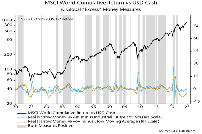
The first indicator is hovering around zero while the second remains negative.

The excess liquidity indicator referred to in the Bloomberg article is described as measuring how much real money growth outperforms economic growth, suggesting that it should resemble the first indicator above. Like here, narrow (M1) money is used in the calculation. Coverage, however, is restricted to the G10 developed markets and growth rates may be measured over 12 rather than six months.

Chart 2 shows a G7 version of the real narrow money / industrial output momentum gap calculated on a 12-month basis, which should be a close substitute for a G10 measure. This indicator turned positive in July but is far from historical highs.

Chart 2

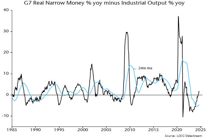
What explains the much more bullish Bloomberg reading? The guess here is that the Bloomberg indicator is a deviation of the real money / economic growth gap from some measure of trend, rather than its absolute level. The current gap, for example, is significantly higher than a 24-month moving average, also shown in chart 2.

In this case, the Bloomberg indicator would be better described as a measure of excess money acceleration rather than growth. The current high reading would reflect a recovery in excess money momentum from deep negative to slightly positive.

Conceptually, it is unclear why the demand for assets should be related to the second derivative of excess money rather than its growth or level. The Bloomberg indicator correctly signalled the strength of equity markets this year, though not in 2023. Backtesting indicates that the sign of an acceleration measure would have underperformed that of the level of excess money growth in signalling whether equity market returns were above or below cash rates historically.

Why did the measures shown in chart 1 “miss” the strength of equity markets in 2023-24?

Excess or deficient money need not affect all markets similarly. Treasuries, commercial property and commodities may have borne the brunt of a money flow shortfall.

Preference for equities has been boosted by the AI boom and associated strength in a small number of large cap stocks. The MSCI World equal-weighted index has underperformed US dollar cash since the excess money indicators in chart 1 turned negative around end-2021.

The key reason for the disconnect with market performance, however, is that the flow measures were, on this occasion, an insufficient guide to the excess money backdrop, failing to take account of a still-large stock overhang left over from the 2020-21 money growth surge.

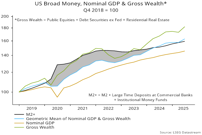
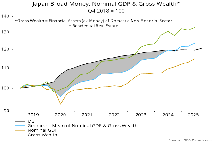
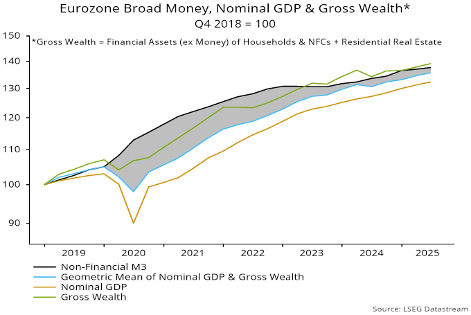
The “quantity theory of wealth”, explained in posts in 2020, is a suggested modification of the traditional quantity theory recognising that (broad) money demand depends on wealth as well as income and proposing equal elasticities. Nominal income is replaced on the right-hand side of the equation of exchange MV = PY by a geometric mean of income and wealth.

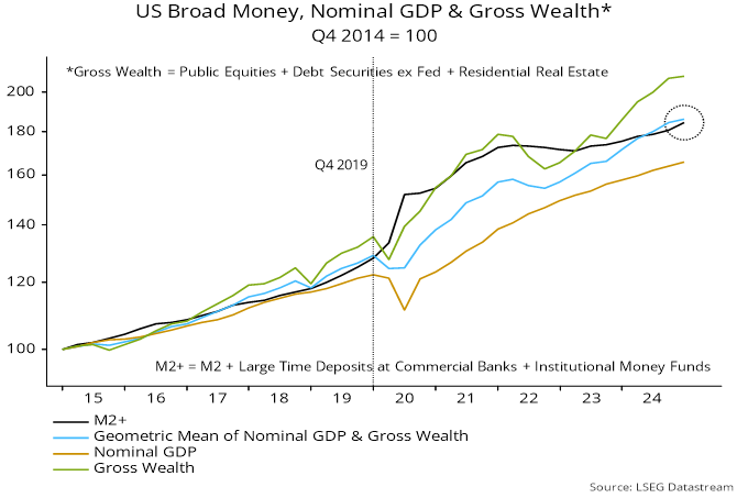
Chart 3 applies the “theory” to US data since end-2014.

Chart 3

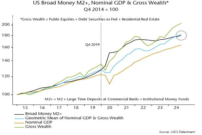
The combined income / wealth variable closely tracked moderate growth of broad money over 2015-19. Wealth rose faster than income, so traditionally-defined velocity fell. The velocity of the combined income / wealth measure was stable.

The policy response to the covid shock resulted in possibly unprecedented monetary disequilibrium. Asset prices responded swiftly to the excess, causing wealth to overshoot broad money in 2021. Excess money flow indicators turned negative around end-2021 and wealth corrected sharply in 2022.

The combined income / wealth measure was still well below the level implied by broad money even before this correction. Deployment of the excess stock fuelled a second surge in wealth from late 2022 while sustaining economic growth despite monetary policy tightening.

Asset price gains, goods / services inflation and real economic expansion resulted in the income / wealth measure finally converging with broad money at end-Q2, with an estimated small overshoot at end-Q3. So the velocity of the combined measure has returned to its end-2019 level.

Stock as well as flow considerations, therefore, suggest that the excess money backdrop is now neutral at best.